HLA*PRG:LA approximates the graph alignment process by starting with linear sequence alignments. It brings down the resource requirements per sample for the HLA typing process to 30GB RAM/30 CPU hours, and produces highly accurate calls.

If you’re interested in immunogenetics, you probably know that high-accuracy HLA type inference from all types of whole-genome sequencing data is now possible: we recently published a tool, HLA*PRG, that enables that.

You might also have noticed, however, that HLA*PRG can be quite resource-hungry – hundreds of CPU hours and up to 80GB of RAM for 2 x 250bp whole-genome sequencing data. Also, it only supported GRCh37.

In this post I describe an algorithm, HLA*PRG:LA, that brings down these requirements to ~30GB and ~30 CPU hours per sample, without sacrificing accuracy.

The “LA” stands for “Linear Approximation”, and this post explains what exactly is being linearly approximated. HLA*PRG:LA is also easier to run than HLA*PRG, and has GRCh38 support.

If you’re not familiar with the HLA and why it is important, have a look at the “HLA primer” at the end of this post.

Population Reference Graphs

Where do the computational demands of HLA*PRG come from? Under the hood, HLA*PRG uses a complex data structure: a Population Reference Graph (PRG). This is necessary because the HLA genes are the most polymorphic genes of the human genome; the HLA region is often referred to as “hypervariable”. When trying to align sequencing reads to the HLA genes, any approach that doesn’t explicitly take this diversity into account is likely to fail and end up misaligning reads to the wrong genes (a full review of the genetic structure of the HLA genes is beyond the scope of this blog post, but one additional factor is that these genes are not only hypervariable, but also strongly homologous, i.e. similar at the sequence level; a single base can make the difference between the exon sequences of alleles belonging to different genes).

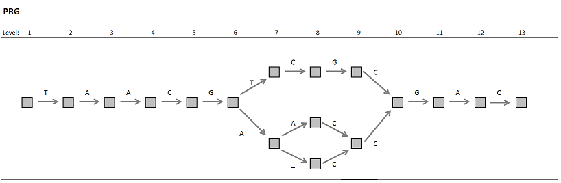
How do PRGs help in genetically complex regions? PRGs explicitly encode the multiplicity of potential sequences in a region of the genome. Typically, a PRG is constructed from a database of input sequences (here: IMGT/HLA, the HLA allele database); and the data structure is a “graph” because the construction algorithm fuses the input sequences at plausible recombination points. You obtain all genomic sequences compatible with a given PRG by enumerating all possible walks through the graph (to keep things simple, the PRGs we use are acyclic and have a structure that resembles – and is indeed derived from – multiple sequence alignments).

Intuitively, if two alleles at different loci are separated by only one SNP, the PRG has the advantage that it “knows” about the existence of these highly similar alleles, and even if this additional information about population sequences is not always sufficient for unambiguously identifying the gene that a read belongs to, it can at least improve the quantification of alignment uncertainty. Here is a little toy PRG with 3 encoded haplotypes:

It should be clear that read alignment to such a graph data structure is intrinsically more complex than alignment to linear sequences; the implementation of HLA*PRG also not very optimized.

Linear sequence alignment to seed graph alignment

With HLA*PRG:LA, we explore a fundamentally different idea: trying to save computational time by “seeding” full graph alignment with linear sequence alignments – this is where the “linear approximation” comes in! Intuitively, if PRGs are constructed from linear input sequences, it should be possible to approximate full graph alignment by first aligning to these linear sequences, and then refining these alignments in full graph alignment mode where necessary. Put differently, the linear seeds will be very similar to full graph alignments, apart from perhaps missed graph recombination points between the input sequences. The approach of HLA*PRG:LA depends on being able to heuristically infer these points from the linear sequence alignments, and switch into full graph alignment where required. One attractive property of this approach is that it leverages highly optimized linear sequence aligners like bwa.

A technical description

So how does HLA*PRG:LA actually work?

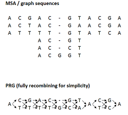
Assume that we have an input MSA and a PRG constructed from the MSA (the graph shown is, for simplicity, fully recombining):

To align a read pair, we go through the following steps (see below for descriptions of the steps):

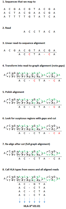
1. Shows the “long” sequences of the PRG that we map to with bwa (for HLA*PRG:LA, this would be the 8 MHC haplotypes plus “genomic” sequences from IMGT; to bwa, all of these sequences are one combined reference genome).
2. Is the read that we want to map.
3. Is one seed alignment of the read to the linear sequences. Reads can (and often have) multiple seed alignments. All of these are taken into the subsequent steps.
4. The seed alignment is projected onto the graph – note the introduction of gaps for consistency with the graph. The alignment path in the graph is shown in green, mismatches are highlighted in red.
5. We “polish” the alignment by, within the coordinate system of the existing alignment, looking for paths that have a higher number of matches than the original alignment. This is necessary because the full PRG has more input sequences than the set that we mapped to; in our case, these additional sequences are the IMGT exonic sequences, and many of the differences between these and the “long” sequences are SNPs. This step makes sure that these SNPs (and small INDELs) get integrated into the alignment.
6. We look for structures, mainly accumulations of gaps, that might indicate that the linear sequence alignment should have crossed a recombination point. We cut the alignment at these points, and retain only the “non-suspicious” component.
7. Switching into full graph alignment mode, we extend the alignment from the cutting points onwards until the complete read is covered. We carry out Steps 3 – 7 for all seeds found for the two reads forming a read pair, and, after having examined and extended all of them individually, find the best pair of graph alignments.
8. After having aligned all reads (here: 5 identical reads), we find the most likely pair of underlying HLA alleles (database search).

This description glosses over some details of the implementation, but gives you a good idea of what is going on.

Performance

How accurate is HLA*PRG:LA?

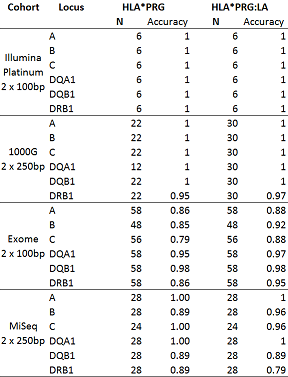
We test the approach on the same datasets that HLA*PRG was tested on, including 5 additional samples from the 1000 Genomes Project. The four test datasets are quite different – two whole-genome datasets with different read lengths; one exome dataset; and one targeted MiSeq dataset. All validation is carried out at G group resolution, which is the resolution often used for clinical typing and which translates into exon sequence (for the exons encoding the binding site of the HLA proteins; see the “HLA primer” for more information). HLA*PRG, and, by extension, this algorithm were designed for whole-genome data – and it is reassuring to see that performance on the whole-genome data is identical, and that performance on the exome data is even slightly improved!

Inferring HLA types for the 2 x 100bp NA12878 sample took 32 CPU hours and 30G of memory; for the 2 x 250bp NA12878 sample, 31 CPU hours and 33G of memory.

Running it!

In most instances, running HLA*PRG:LA should be as simple as:

./inferHLATypes.pl --BAM /path/to/indexed.bam --graph PRG_MHC_GRCh38_withIMGT --sampleID mySampleID

, where indexed.bam is a GRCh37- or GRCh38-mapped BAM or CRAM file.

HLA*PRG:LA and HLA*PRG

Are there situations in which we would expect the original HLA*PRG to outperform HLA*PRG:LA, or vice versa? Conceptually, I view graph alignment as the “right” approach to the problem of HLA typing, and indeed there are some additional heuristics required to make HLA*PRG:LA avoid mismappings. It might be that some of these heuristics are less robust when applied in the context of highly diverged samples. Ultimately, the relative performance of the approaches is of course an empirical question – we’d love to hear from you if you have additional benchmarking data! Remaining challenges There are some important challenges that we haven’t addressed yet with HLA*PRG:LA:

1. Typing resolution. The two HLA*PRGs operate at G group resolution (exons 2/3 for class I HLA genes and exon 2 for class II HLA genes). Eventually we’d like to bring this up to full 4-field resolution (complete genomic sequence).
2. Novel alleles. Eventually we’d like to be able to call them, and extend databases like IMGT/HLA with population calls.
3. Long reads. It would be nice for HLA*PRG:LA to work on Nanopore and PacBio reads.

Repository and citation

https://github.com/AlexanderDilthey/HLA-PRG-LA/

If you use HLA*PRG:LA, please cite the original HLA*PRG paper.

A quick HLA primer: Relevance, function, genetics and HLA types

From a biomedical perspective, the HLA genes are probably the most important gene family in the human genome. They are also among the most complex loci of the genome, and this is not a coincidence.

Historically, medicine has used the HLA system to practice genetically informed “personalized medicine” long before the term “personalized medicine” became popularized: whether a donor-recipient pair for bone marrow transplantation is compatible is determined largely by their HLA types, and we have large international databases of willing donors and their HLA types that are queried whenever a transplant is required.

Also, an individual’s HLA types influence which “antigens” (things that the immune system can respond to) become visible to immune cells – and this, in turn, has a significant influence on individual disease risk and pharmacogenomics. In many genome-wide association studies, in particular of autoimmune diseases, the HLA region accounts for the by far most significant effects! In addition to predicting and understanding individual disease risk, HLA types will also play an important role in designing individualized immunotherapeutic interventions. In cancer patients, for example, the immune system can be primed against the antigen-inducing mutations that distinguish the tumor from normal body cells – an approach referred to as “personalized therapeutic vaccination”. The first step of the vaccine design process is distinguishing between mutations that are immune-visible (i.e. antigenic) and -invisible, and this is an HLA-driven process – only peptides that bind well to an individual’s HLA proteins are visible to the immune system (and see below for some more details on this)!

Function

On a functional level, the HLA proteins fulfil a range of important immune system functions:

First, they serve as markers of “self” against “non-self” – “self” cells can, broadly speaking, be expected to express the “right” types of HLA markers on their cell surfaces.

Second, they provide an interface for immune cells to inspect the inner workings of body cells (fulfilled by the “class I” HLA proteins). HLA class I proteins are manufactured inside cells and migrate to the cell surface, where they display themselves to immune cells. Before they migrate, however, they pick up random amino acid chains (peptides) from the inside of the cell. Bypassing immune cells can then interrogate the patterns of HLA-bound peptides on the cell surface for hints of anomalous processes. As an example, consider that a replicating virus takes over a cell; the assembly process of new viruses inside the cell comprises steps of peptide synthesis, and some of the virus-specific peptides will, via the random sampling process, end up on the cell surface – where they are visible to, for example, immune cells that can respond by killing the infected cell.

Third, they provide an interface for the coordination of immune cells (fulfilled by the “class II” HLA proteins). Class II HLA proteins are, generally, used to present peptides from materials of external origin (relative to the cell with class II HLA); for example, if a macrophage engulfs and phagocytoses a bacterial cell or a virus, peptides from the bacterial cell or virus will end up (in HLA-bound form) on the surface of the macrophage! Again, the immune system can scrutinize these HLA-bound amino acid chains on the macrophage (or other so-called “antigen-presenting cells”), and modify the behavior of the macrophage accordingly. For example, if the patterns are indicative of a viral infection that the immune system is currently fighting against, other immune cells in the proximity can “activate” the macrophage and increase its effectiveness.

It should be pretty clear by now that any pathogen or pathological process that manages to evade HLA presentation has a selective advantage (the HLA proteins have biochemical “binding preferences” – they can only present a subset of all possible peptides)! This is reflected in a myriad of evolutionary strategies; for example, certain viruses deactivate the cellular expression of HLA proteins; HIV mutates in vivo to better escape immune surveillance, i.e. “away” from the presentational preferences of an individual’s HLA proteins; cancer cells undergo “immunoediting”, a phase during which the most mutagenic mutations in a cancer genome are selectively eliminated.

Diversity as evolutionary strategy

The diversity and genomic complexity of the HLA system, then, is our evolutionary counter-strategy! This plays out on at least two different levels. First, population polymorphism: if you are a pathogen and your survival strategy is to mutate in a manner that makes you invisible to an individual’s immune system in a HLA-dependent manner, you are in trouble if the next person you’d like to infect has HLA proteins that are structurally very different from your current host!

Second, within-genome HLA complexity: even if there is a lot of HLA polymorphism in a population, you could still try to adapt to an individual’s HLA types upon each new infection event, if you’re just fast enough to avoid being killed before you’re adapted. The probability of this strategy of within-individual adaptation being successful, however, becomes smaller as individual immune systems become more structurally and genetically complex. A haploid human genome has 3 “classical” HLA class I genes (HLA-A, -B, -C) and 3 “classical” class II genes (HLA-DQA1, HLA-DQB1, HLA-DRB1); and all of these genes are very polymorphic in the human population, e.g. HLA-B with >4000 known alleles. A typical individual genome might therefore contain, for example, 11 different class I and 10 different class II sequences – adapting to all of these protein structures simultaneously might be impossible or at least place you under strict evolutionary constraints, which might reduce your genetic fitness.

From a perspective of genome evolution, the HLA genes are a “birth-and-death” gene family; on evolutionary timescales, some genes “die” as they degenerate into pseudogenes (the human genome contains quite a few HLA pseudogenes); and new genes are “born” by gene duplication events. Both shared origin and similar functionality therefore account for the observed sequence homologies between alleles of different HLA genes!

HLA types

Finally, what about “HLA types”? HLA types are a nomenclature system that assigns a unique code (“HLA type”) to each catalogued HLA allele; nowadays, “allele” is usually understood as “genomic sequence at a locus”. HLA types are named according to a specific scheme; details are explained on the IMGT/HLA website, or in the HLA*PRG paper.

The most popular resolution of HLA types nowadays is “G group” resolution. Each allele at G group resolution defines the sequences of the “most important” exons of an HLA gene (“most important” means exons 2 and 3 for class I genes and exon 2 for class II genes; these exons account for most of the peptide-binding variabilities associated with different alleles). IMGT/HLA maintains a list of G group alleles and how they relate to alleles at other resolutions.

HLA*PRG and HLA*PRG:LA infer alleles at G group resolution; that is: they give you the sequences of the exons that encode the HLA protein binding site. Most of the validation data utilized here is also at G group resolution.