The T2T-CHM13v2.0 release includes complete assemblies for all 24 human chromosomes. Chromosomes 1-22 and X are from the CHM13hTERT cell line and chromosome Y is from NIST HG002 (aka PGP huAA53E0). The CHM13 chromosomes are described in the below linked publications, and we expect to release a preprint on the HG002 chrY within the coming month. This data is released into the public domain without restriction. We politely request that you cite Nurk et al. “The complete sequence of a human genome” for its use.
Science special issue “Completing the human genome”
T2T companion papers at Science, Nature Methods, and Genome Research
UCSC Genome Browser (chm13)
NCBI GenBank Record (GCA_009914755.4)
Ancillary data (GitHub)
In addition to the NCBI assembly record, we are providing the following FASTA files for convenience.
chm13v2.0.fa.gz
CHM13v2.0 reference with repeats soft-masked and sequence names converted to the UCSC style
chm13v2.0_noY.fa.gz
CHM13v2.0 excluding the Y chromosome
chm13v2.0_maskedY.fa.gz
CHM13v2.0 with the Y pseudoautosomal region (PAR) hard masked with Ns
chm13v2.0_maskedY_rCRS.fa.gz
CHM13v2.0 with the Y pseudoautosomal region (PAR) hard masked with Ns and the CHM13 mitochondrial genome replaced with the rCRS reference
A huge thank you and congratulations to all the members of the T2T consortium! There are 100 co-authors of the assembly paper, and many more who have contributed to our understanding of the first complete human genome. I cannot show them all here, but hopefully this montage will give you a feel for the incredible team that made this dream a reality.
]]>Multiple positions are available under the supervision of Dr. Adam Phillippy at the NIH’s National Human Genome Research Institute (NHGRI). Dr. Phillippy leads the Genome Informatics Section, which develops and applies computational methods for the analysis of massive genomics datasets with a focus on problems related to genome sequencing. Members of the section have developed many widely used bioinformatics methods (e.g. MUMmer, Mash, Canu), and are leaders in the field of long-read DNA sequencing.
The section is currently seeking applicants with an interest in developing and/or applying computational methods for genome assembly, sequence alignment, structural variant detection, metagenomics, and information visualization. Current projects in the lab include our efforts to finish the human reference genome (Telomere-to-Telomere Consortium), sequence and explore the human pan-genome (Human Pangenome Project), and assemble the genomes of many diverse vertebrate species (Vertebrate Genomes Project). Future work includes democratizing genomics with real-time nanopore sequencing and analysis. Applicants must possess strong English, programming, and analytical skills. Past experience in computational genomics is preferred but not required.
The NHGRI Intramural Research Program is located on NIH’s main campus in Bethesda, Maryland and offers a wide array of training and collaboration opportunities for early-career scientists. The funding for these positions is stable and offers wide latitude in the design and pursuit of bioinformatics research. The successful candidate will have access to extensive high-performance computing resources (BioWulf), the NIH intramural sequencing center (NISC), NHGRI core facilities, and the NIH Clinical Center. The typical stipend for a computational postdoc is approximately $70k per year and includes family health insurance. Software engineering salaries are commensurate with experience and competitive with industry. Answers to some frequently asked questions can be found here: NIH Postdoc FAQs. PhD training can also be arranged through most nearby universities, such as the University of Maryland, via the NIH Graduate Partnerships Program.
To apply: Interested applicants should submit their CV, a brief personal statement, and the names of three references to: adam.phillippy@nih.gov
The NIH is dedicated to building a diverse community in its training and employment programs.
]]>Roughly twenty years ago, the International Human Genome Sequencing Consortium published an “Initial Sequencing and Analysis of the Human Genome” simultaneously with “The Sequence of the Human Genome” from Celera Genomics. Although the public consortium chose a more humble title that suggested some work was left to be done, amidst all the pomp it was easy to miss the fact that the human genome had not actually been finished. The key caveat appears early on in both papers, e.g. “A 2.91-billion base pair (bp) consensus sequence of the euchromatic portion of the human genome was generated”. Ignoring heterochromatin, due to difficulty in mapping, cloning, or assembling these sequences, excluded upwards of 10% of the genome from these initial drafts, and that missing fraction has been underappreciated ever since. Today, the latest human genome reference (GRCh38) still contains 161 Mbp of “unknown” sequence constituting 5% of the genome.
Now, twenty years later, we are finally able to fill in the blanks thanks to a confluence of new sequencing technologies from PacBio and Oxford Nanopore. Within the past year, the T2T consortium assembled the first complete human chromosomes, Chromosome X and Chromosome 8, using Nanopore ultra-long (UL) sequencing as a backbone and polishing that sequence with PacBio and Illumina. However, the recent release of PacBio’s HiFi technology led us to revise our recipe. In the assembly presented here, we first constructed a highly-accurate assembly graph using PacBio HiFi reads and then resolved any structural ambiguities with the help of Nanopore UL reads. The following image shows a Bandage visualization of our HiFi string graph for the CHM13 genome, with most chromosomes resolved as individual components.
After resolution of the remaining “tangles” with the help of Nanopore UL reads, the sequence of each complete chromosome was obtained via a consensus of HiFi reads taken from the corresponding traversal of the graph. This approach allowed us to reach T2T continuity for all chromosomes, while retaining the accuracy of PacBio HiFi throughout. Nanopore data also helped by patching a few regions of the genome that PacBio failed to sequence due to an apparent sequencing bias in GA-rich repeats. Similar graph-based hybrid approaches have previously been used to combine Illumina and long-read sequencing data for microbial genomes, but this has not been possible for human genomes due to the larger genome size and higher repeat complexity. However, because HiFi reads are both long and accurate, the complexity of the resulting HiFi graph is tremendously reduced compared to Illumina, allowing for complete resolution of the remaining tangles via Hamiltonian paths and, in the worst cases, Nanopore threading.
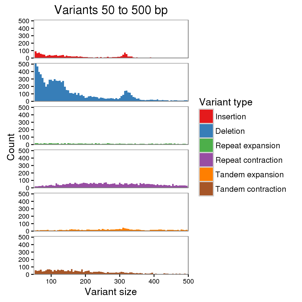
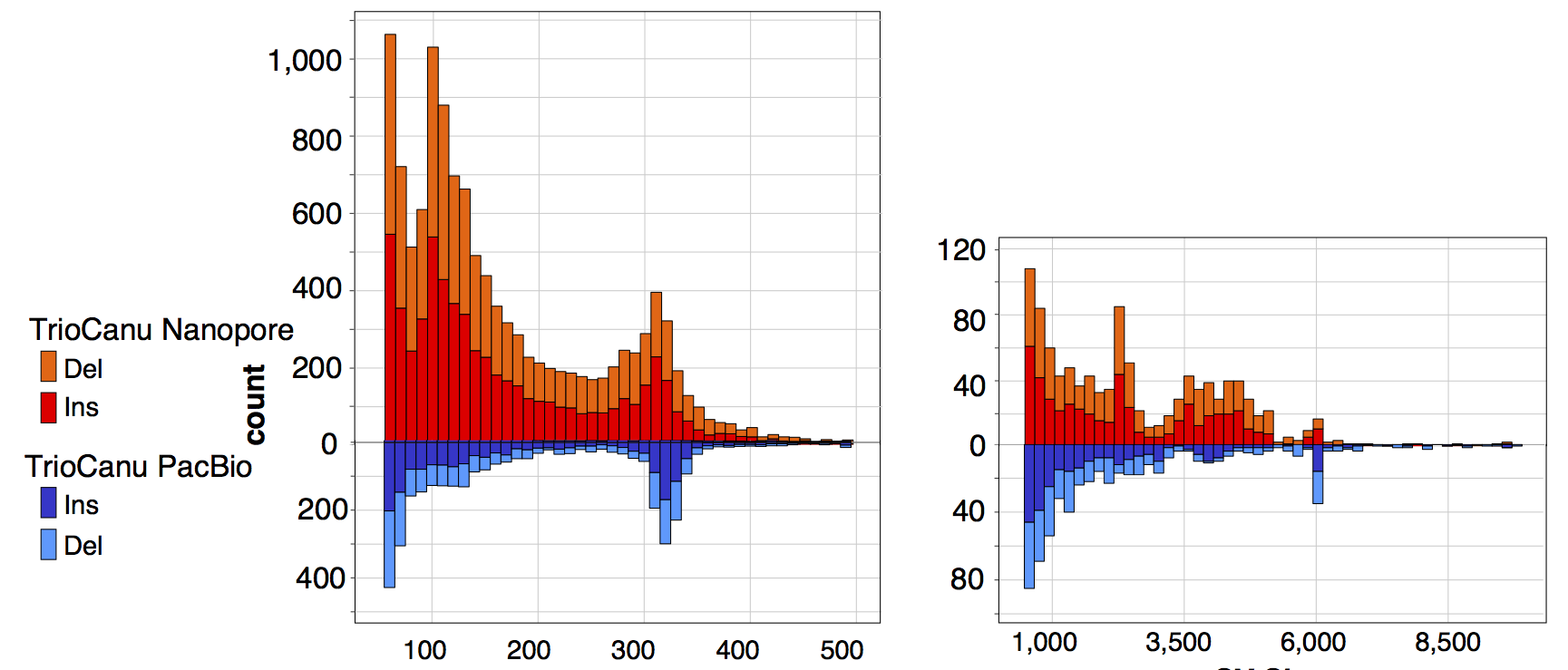
We estimate that the consensus quality of our HiFi-based assembly exceeds Q60 (less than 1 error per million bases), with most remaining errors localized to homopolymers, which is a known issue for both PacBio and Nanopore sequencing. To correct homopolymer errors and further improve quality, we mapped the raw PacBio, Nanopore, and Illumina reads to our initial assembly and called variants using DeepVariant and Sniffles. Considering only the most confident variant calls (likely to be assembly errors, rather than heterozygosity), we made a total of 4 structural corrections and 993 small variant corrections. We estimate that the quality of our polished assembly approaches Q70 (1 error per 10 million bases), with no known structural errors. We plan to continue scrutinizing the assembly over the coming months and will generate updated versions to correct any errors identified.
Both the v0.9 pre-polished and v1.0 polished assembly are now freely available for download. The CHM13 cell line possesses a 46,XX karyotype with almost complete homozygosity between chromosome pairs. As such, the v1.0 assembly contains 23 chromosomes (no ChrY) and 1 mitochondrial genome totaling 3,045,441,522 bp of assembled sequence. A small number of heterozygous variants were observed in the genome and will be fully cataloged in a future release. As mentioned above, only the 5 rDNA arrays remain unfinished. Some full and partial rDNA units are assembled on each of the 5 acrocentric p-arms, but the centers of these arrays are currently represented by a total of 11.5 Mbp of Ns in the assembly (on Chromosomes 13, 14, 15, 21, 22). Because the rDNA arrays are near-identical tandem repeats, the content of these arrays is known and only the contained variants remain to be determined. We expect to finish these arrays and add a Chromosome Y (from a different cell line) in the coming year.
Due to our rapid release timeline, many details of our methods and validation have been omitted here. We plan to post a preprint fully describing this project in the coming months, and our consortium is in the process of characterizing these newly uncovered regions of the genome. We have freely released all of our raw data and assemblies without restriction, but ask as a courtesy that you contact us if you would like to contribute analyses prior to our initial publication of results in approximately 6 months. The T2T is an open consortium and all are welcome to join our effort to generate the first truly complete assembly of a human genome. If you would like to join us, please contact T2T co-chairs Adam Phillippy adam.phillippy@nih.gov and Karen Miga khmiga@ucsc.edu to be added to our mailing list.
Who is the T2T consortium? You can find a continually updated list of contributors on our members page. I would like to sincerely thank everyone involved for their dedication over these past few months. An incredible amount of work was accomplished in a very short time. Thanks also to our industry partners at PacBio, Oxford Nanopore, Arima Genomics, Amazon Web Services, and DNAnexus who helped enable this work.
I would especially like to thank the working group co-chairs who helped me organize this summer’s finishing workshop: Sergey Nurk (assembly), Karen Miga (satellite DNAs), Arang Rhie (polishing and validation), Mark Diekhans (browser and annotation), Mitchell Vollger (segmental duplications), and Justin Zook (variant calling). Sergey Nurk deserves special credit for developing the HiFi assembly methods that enabled such rapid progress this year.
Lastly, I would like to acknowledge an abbreviated list of software that was critical to the success of this project: HiCanu, Miniasm, Winnowmap, Minimap, GraphAligner, MUMmer, CentroFlye, TandemTools, StringDecomposer, Bandage, GFA, IGV, DeepVariant, Merqury, and SDA. In particular, the contributions of Heng Li in terms of both tools and formats have been invaluable. Never forget that the field of genomics is entirely dependent on free software and the developers of these tools deserve endless thanks and support!
Stay tuned for much more to come from the T2T consortium this year as we begin to analyze these new sequences of the human genome. For now I will just leave you with a teaser dot plot of all ≥50 bp exact repeats within a novel 3 Mbp region on the short arm of human Chromosome 14, which I think looks quite beautiful (fwd in purple, revcomp in blue).
]]>We started by re-calling the raw data using Albacore v2.1 with default parameters. The total coverage increased from 37X to 41X. A free 4-fold coverage increase from a software update, not bad! The average read length also increased from 7.3 to 8.1 kbp. Re-assembling with Canu 1.6 gave an improved NG50 of 10.2 Mbp and required approximately 150k cpu hours, as in the paper. We also assembled the genome using a combination of Canu 1.7 read correction with WTDBG contigging. This further increased the NG50 to 12.4 Mbp due to improved read correction in Canu 1.7, and required 30k cpu thanks to the speed of WTDBG. There is still room for improvement with coverage or longer reads since the most continuous human assemblies are over 20 Mbp. The Cliveome is currently the most continuous, with an NG50 of 29 Mbp from a high-coverage combination MinION and GridION data.
The Canu + WTDBG assembly is more continuous than either a Miniasm assembly (NG50=6.7Mbp, 8k cpu with Racon) or a WTDBG-only assembly (NG50=8.7Mbp, 0.5k cpu), neither of which perform read correction. Thus, Canu’s read correction does appear to benefit assembly and we plan to make this Canu + WTDBG pipeline available in a future Canu release. In the meantime, users can run the Canu correction module and feed its output directly into WTDBG for a faster assembly option.
We also evaluated the base quality of the new Canu + WTDBG assembly. The identity is 98.94%, up from the 95.94% we previously reported. This also improves upon the 97.80% identity we reported for a chromosome 20 assembly of Scrappie-called reads (Jain et al. 2018). After two rounds of Nanopolish with its new “CpG methylation” mode, the Canu + WTDBG assembly identity improved to 99.76%. We still see a deletion bias and a high fraction of short indels, but a peak for Alu indels is clearly visible now, whereas it was not before. We are encouraged by these improvements.
However, 99.76% is still a bit disappointing. It is much better than 95.94%, but represents an error about every 400 bp. Commonly, Illumina data is used to polish away this remaining 0.25% of error, but this has its own issues, especially for heterozygous genomes and complex repetitive regions where short-read mapping is a challenge.
Because parental data is available for GM12878, we also attempted complete haplotype assembly using our recently described trio binning approach (Koren et al. 2018). Using TrioCanu, we classified the nanopore reads for GM12878 into maternal and paternal haplotype bins prior to assembly. Despite the lower coverage (40x Nanopore vs. 70x PacBio), we saw a similar classification rate (85% of bases classified by haplotype) and similar NG50 stats for the assembled haplotigs (1.3 Mbp paternal, 1.2 Mbp maternal). The identity for both haplotypes after two rounds of CpG Nanopolish was 99.24%. Consistent with our results on other datasets, we would expect both larger NG50s and higher identity with more coverage. In this case, Nanopolish is dealing with less than 20x coverage per haplotype.
We also aligned the two nanopore haplotypes to one another to call structural variants and compared these results to the same analysis performed with PacBio:
There are again more short indels than expected in the Nanopore assembly (presumably due to base-calling biases and the lower depth of coverage). In comparison, the PacBio haplotypes show more concentrated SV peaks at the typical Alu and LINE sizes (300bp and 6kb). Repeating the MHC analysis from our trio binning preprint, the HLA typing genes in both nanopore haplotypes are correct at G-level resolution and properly phased, with an average edit distance of 1 bp per gene (12 errors total). This is better than the 10x Genomics result but worse than the PacBio result presented in the preprint.
Highlighting the difficulty of polishing complex regions with Illumina data, attempting to run Pilon on each nanopore haplotype using the parental Illumina data actually reduced the quality and introduced additional errors in several MHC genes. However, restricting Pilon to only correct indels did fix all typing gene errors and yielded a final consensus accuracy of 99.92%. (Note that this experiment was only for evaluative purposes, and naive polishing with parental data runs the risk of masking de novo variants in the child.)
Oxford Nanopore continues to make impressive strides. Recent software improvements (primarily for base calling) have almost doubled the assembly NG50 size for the GM12878 assembly, without the addition of any new data. In parallel, we are continuing to work on Canu performance and in the meantime recommend Canu + WTDBG as good compromise between speed and accuracy. Extremely continuous assemblies are clearly possible using long-read nanopore data alone. The last remaining hurdle is final consensus accuracy, which continues to come up short of PacBio and requires additional polishing using complementary data (e.g. Illumina) to reach “reference” quality.
Nanopore data also appears well-suited for trio binning. For long-read reference genome assembly, we now suggest collecting parental Illumina data wherever possible. This approach greatly simplifies the assembly of heterozygous genomes and yields accurate representations of both haplotypes. If performed on a hybrid cross, this method will yield two reference genomes from a single sequencing project, as we recently demonstrated using a cattle F1 cross. Human trios can be harder to come by, but the method is applicable and works well for reconstructing heterozygous structural variation.
Finally, a note of caution on Illumina polishing with Pilon. While it can improve consensus statistics overall, it can worsen the assembly in some regions, especially complex repetitive sequence like the MHC. If using Pilon, we recommend limiting the allowable edits and focusing on the primary nanopore error mode (indels). Using a purpose-built variant caller instead, such as FreeBayes, is also advisable but requires custom editing of the consensus. A more sophisticated approach to hybrid Nanopore + Illumina assembly would be ideal, but we have not yet seen a satisfactory solution. Ultimately, resolving the last bit of nanopore error without an additional technology would be best, and it will be exciting to see if Oxford Nanopore can achieve this with future updates to sequencing and/or base calling methods.
You can find a description of our assembly methods in the Jain et al. 2017 paper and the trio binning paper Koren et al. 2018. Sergey will be presenting this work at London Calling this week.
Update 2018-05-24: The basecalled data is available from the NA12878 consortium. Update 2018-05-29: We’ve made the basecalled data split into maternal, paternal, and unclassified bins available. Update 2018-10-28: We’ve made the Canu + Nanopolish + Pilon + Racon assembly, which is 99.99% identity, available. Download the Canu 1.7 + WTDBG + Nanopolish assembly or the maternal and paternal assemblies.
]]>We have been working on the containment problem since this spring, but were holding back a new Mash release until we could get the accompanying paper written. However, David Koslicki and Hooman Zabeti recently posted a preprint with similar ideas, so we decided to make the new Mash release available and write this short blog in the interim. The following is a brief description of “containment” and the available techniques for computing it.
Consider two k-mer sets A and B with the above Venn diagram. Biologically, this could represent a plasmid A contained in a genome B, or a genome A contained in a metagenome B. In either case, the resemblance of these two sets is low because there is a large amount of B that is not in A, yet A is perfectly contained in B. This distinction is reflected in the denominators of the respective formulas:
Thus, containment reports what fraction of A’s k-mers also appear in B. As we describe below, this measure can be estimated very efficiently and has some obvious applications in metagenomics.
Mash uses a MinHash bottom sketch to rapidly estimate the resemblance of two genomes (or metagenomes). A bottom sketch is simply a set of the s smallest hash values seen after hashing all k-mers in a genome. Given the mathematical similarity between resemblance and containment, it is tempting to use the same structure to estimate both. However, as Broder noted in his original paper, a bottom sketch is poorly suited to estimate resemblance. The reason is illustrated here with three genomes {a,b,c} that are components of a metagenomic mixture:
A bottom sketch of four elements is shown (in red) for the three toy genomes and the mixture. In this case we would miss the matching ‘10’ from genome c because it is not included in the bottom sketch of the mixture. Smaller sets, like c, tend to have a wider range of values in their bottom sketch since there are fewer hashes to choose minimums from. Because all the sketches are of a fixed size, these larger hash values get bumped out of the larger mixture sketch. To account for this, Broder originally proposed using modulo operations to build sketches meant for containment estimation. In this way, individual sketches can grow with the size of the sets. For example, using modulo 2 would build sketches of only even hashes (in red):
With a sketch of modulo 2, the match of ‘10’ between c and the mixture would be recovered. However, now the sketch sizes are no longer fixed and grow linearly with genome size. This sacrifices much of the memory and storage of the MinHash technique.
The Koslicki and Zabeti preprint includes a nice exposition of why MinHash sketches are problematic for estimating containment, and provides examples of how the relative error of this technique explodes when the size of A is much smaller than B. However, as Broder stated in his 1997 paper, MinHash was never intended for this purpose (some words substituted to match the terminology of this post):
The [MinHash sketch] has the advantage that it has a fixed size, but it allows only the estimation of resemblance. The size of [the modulo sketch] grows as [the set] grows, but allows estimate of both resemblance and containment … The disadvantage of this approach is that the estimation of the containment of very short documents into subtantially [sic] larger ones is rather error prone due to the paucity of samples.
This last point is why the modulo approach is problematic for metagenomic applications (e.g. finding a virus in a metagenome). A small modulus would be required to detect the virus, and as a result the sketch of the metagenome would be huge. Instead of the modulo approach, Koslicki takes a MinHash sketch of the k-mers from genome A and a bloom filter of k-mers from (meta)genome B. To estimate the containment of A in B, one simply looks up all of the hash values from the sketch of A in the bloom filter of B. From this, one can estimate containment after accounting for false-positives arising from the bloom filter membership query. Here it would have been nice to see a comparison versus Broder’s modulo approach. To assure a low false-positive rate, bloom filters can require a large amount of space. For the same error bounds, does the bloom filter save substantial space over the modulo approach? Unfortunately, Koslicki does not reference the modulo technique.
Screen is a new command offered by the Mash toolkit that also answers the containment question. Many of our users wanted to use Mash to quickly determine the composition of their sequencing runs (e.g. for contamination screening), but we knew that the standard MinHash approach was not ideal for this. Like Koslicki, we observed that it was possible to repurpose the reference genome sketches to answer this question, and we already had a sketch database for all of RefSeq. However, rather than use a bloom filter, we use an exact, streaming method to identify which sketch values are found in the sample. Since each sketch is effectively a random sample of the k-mers in a genome, the containment of each genome A in B is simply the fraction of matched values in the sketch of A.
Implementing the streaming approach is straightforward. Because the sketches themselves are quite small (the all RefSeq sketch database is only around 100 MB), it is possible to store a hash table of all sketch values in memory. Then, a set of sequencing reads can be streamed as input and every k-mer quickly checked against this hash table. Each time a k-mer is seen that maps to a sketch element, a counter is incremented using atomic types to support multi-threading. The resulting count table allows us to estimate the containment of every genome in the database, and also provides a rough depth of coverage estimate for each. One advantage of this approach is that it is “online”, meaning the containment and coverage values can be continuously updated during a real-time sequencing run.
Overview of Mash Screen. (A) A set of reference genomes is processed to produce a (B) sketch database. (C) A hash table of all sketch elements is used to count occurrences in (D) a streaming sequencing mixture. For each genome, (E) the fraction of the sketch observed in the mixture produces (F) a containment estimate.
This new function also includes support for translated blastx-style operations. When calling screen against a protein database, Mash will automatically perform six-frame translation on the input nucleotide sequences. This could be handy for quickly computing containment of viruses or individual genes within metagenomes.
The latest Mash release can be grabbed from here. The new screen operation is compatible with the existing RefSeq sketch database, or a custom database can be created for any collection of sequences (nucleotide or protein). A set of sequencing reads can then be streamed against this database requiring just a few minutes per thread per gigabase of reads:
mash screen RefSeqSketches.msh reads1.fastq reads2.fastq > out
Also check out David Koslicki’s CMash for the bloom filter implementation of containment. A potential advantage of the bloom filter approach is that it could enable indexed search of a bunch of metagenomes. For example, given an indexed database of metagenomes, one could ask the question “In which metagenomes has this new genome been seen before?” Conversely, due to its streaming nature, Mash screen is best suited to answer the question “Which genomes are contained in this new metagenome?” Both tools should be handy for searching large databases, quick contamination checks, and as a pre-filter for read classification. For example, one could run a containment check first and then map reads only to those genomes identified.
Here are the first 10 lines of output for SRA sample SRS1041159 (tongue dorsum) “screened” against all of RefSeq genomic:
0.997007 939/1000 12 0 Human endogenous retrovirus K113 (viruses)
0.995206 904/1000 53 0 Neisseria flavescens (b-proteobacteria)
0.995206 904/1000 27 0 Haemophilus sp. HMSC061E01 (g-proteobacteria)
0.994784 896/1000 28 0 Haemophilus sp. HMSC068C11 (g-proteobacteria)
0.994199 885/1000 27 0 Rothia sp. HMSC061C12 (high GC Gram+)
0.99339 870/1000 27 0 Rothia sp. HMSC065C12 (high GC Gram+)
0.992899 861/1000 29 0 Rothia sp. HMSC065B04 (high GC Gram+)
0.992844 860/1000 28 0 Haemophilus parainfluenzae (g-proteobacteria)
0.992844 860/1000 25 0 Haemophilus parainfluenzae (g-proteobacteria)
0.992789 859/1000 30 0 Rothia sp. HMSC066G02 (high GC Gram+)
The output columns are [identity, shared-hashes, median-multiplicity, p-value, query-ID]. There are many more lines following, including human further down the list:
0.955446 384/1000 1 0 GCF_000001405.36_GRCh38.p10
A couple things to note. First, the identity score is not the true identity of a genome versus what is in your sample, but what fraction of bases are shared between the genome and your sequencing reads (this is estimated from the fraction of shared k-mers). Sequencing errors and gaps in coverage will reduced the identity estimate. For example, since the human genome is in the sample at low coverage, not all human k-mers are found and the corresponding identity score is reduced.
Second, Mash Screen is not a metagenomic profiler in the traditional sense. When using a comprehensive sketch database there is typically a lot of redundancy in the output. The tool is simply reporting every genome in the database that shares a high fraction of k-mers with the sample. In this example, some microbial genomes are high coverage and so hits pop up to all strains that are similar (e.g. multiple Haemophilus genomes). It is very unlikely that all reported strains are actually there, but Mash is not yet attempting to answer which ones are. It would be great to see additional methods developed to process containment scores, reduce the output redundancy, and report accurate compositional estimates for metagenomes. One easy approach is a “winner take all” model, like sourmash implements. This is now available in Mash as an option to the containment function, but much better methods are possible and left for future work. Check out MetaPalette for some possible inspiration.
We hope you will find these tools useful!
]]>